The returns we want | Part 1

In yesterday’s introduction we asked a simple but fundamental question: if we could design a money machine to generate returns for us, what would we want it to look like?

This first part begins with the foundations. Before we can talk about uncertainty, preferences, or practical heuristics, we need to understand what kinds of profit and loss streams emerge from different assumptions about the return-generating process.

We will explore three core features:

• Diversification and the Central Limit Theorem. How combining many independent bets reduces risk and normalises distributions, and why this is often called the only free lunch in finance.
• Compounding and path dependence. How the sequence of gains and losses shapes long-term outcomes, and why geometric returns behave so differently from arithmetic averages.
• Dependencies across assets and time. How correlation, autocorrelation, and volatility clustering reduce the effective number of independent bets and weaken diversification.

By simulating these effects and illustrating them with simple models, we can see how core statistical structures shape the behaviour of a money machine. This sets the stage for Part 2, where we will move from modelling the process itself to addressing our uncertainty about its parameters and how we learn about them over time.

Simulating Profit and Loss (P&L) Streams

The only free lunch

The money machine is a dynamic process that makes trading decisions and manages positions in response to signals and portfolio logic. This process can be measured at a chosen temporal resolution (e.g., daily), resulting in a time series of profit and loss (P&L) or returns. Each daily return is the aggregate outcome of many underlying strategies and signals, each contributing a random component to the day’s result.
The first analytical question is therefore: What is the shape or distribution of these aggregate daily returns?
When describing distributions, finance professionals pay close attention not only to the mean (average return) and standard deviation (risk or volatility), but also to higher moments: skewness and kurtosis. Skewness describes the asymmetry of the distribution: a strategy with positive skew may offer occasional large gains but more frequent small losses (as in the case of a lottery ticket—many small losses, rare big wins, and a negative average return). Kurtosis, or “fat tails,” reflects the probability of extreme outcomes: distributions with high kurtosis feature more frequent large surprises than the normal bell curve would suggest. Insurance strategies, for example, may be designed to protect against such rare but severe events.
Combining many independent “daily bets” in this way leads to what, in the finance profession, is sometimes called ‘the only free lunch’: diversification, as formalised by the Central Limit Theorem.
The Central Limit Theorem states that if we add together a large number of random variables that (i) are drawn from the same distribution, (ii) are independently sampled (a requirement we will return to), and (iii) have finite variance, then as the number of independent bets approaches infinity, the resulting sum distribution converges to a normal distribution.
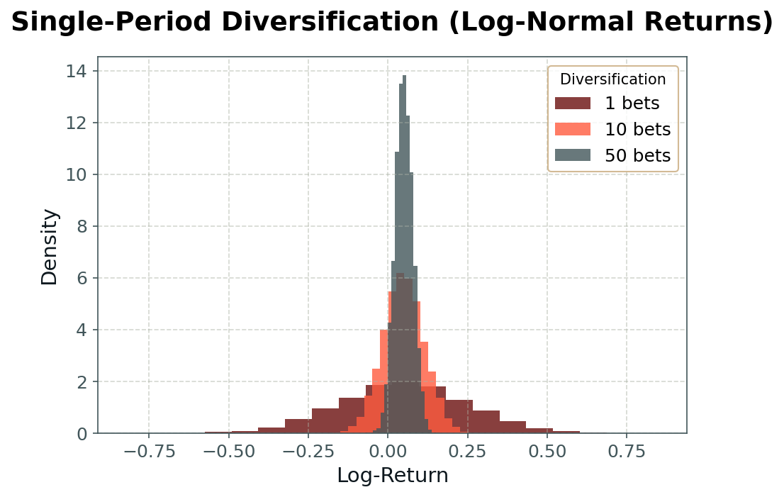
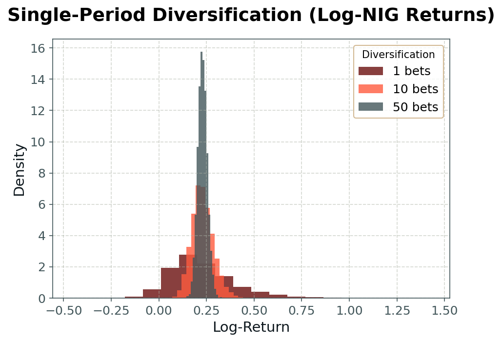
We can demonstrate the effect of the CLT in the practical context of our money machine by simulating daily returns constructed as averages across nnn independent bets, each drawn either from a normal distribution (as shown in Fig. 1) or from a normal-inverse Gaussian (NIG) distribution (Fig. 2). As we increase the number of independent sub-strategies, the aggregate return distribution becomes narrower (i.e., risk declines), and—especially in the case of non-normal atomic distributions—more ‘bell-shaped.’
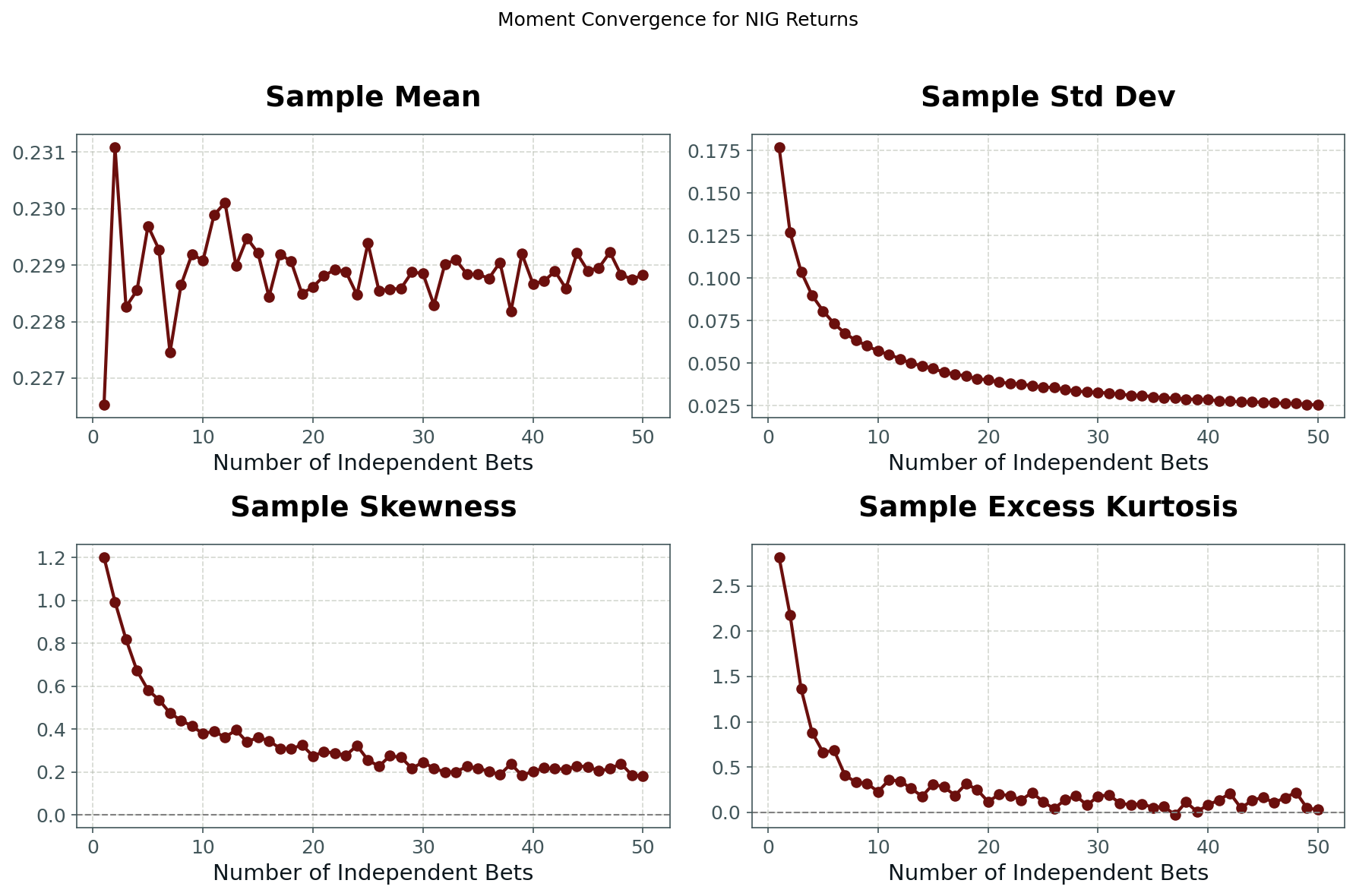
In Fig. 3, we illustrate this effect quantitatively by plotting the first four moments (mean, standard deviation, skewness, excess kurtosis) of the aggregate returns as a function of nnn for NIG-distributed sub-strategies. We observe that the mean remains unchanged, while the variance, skewness, and kurtosis all decline as the number of independent bets increases.
This is the essence of diversification: aggregating across many positions leads to less risky, more predictable, less skewed, and less tail-heavy outcomes. It is the fundamental principle underlying the insurance industry, and it explains the scale effects in finance—why large, diversified portfolios so often outperform small, concentrated strategies.

Time bites back

The money machine does not produce returns in a single period; rather, it generates a continuous stream of profit and loss over time. How these returns accumulate, whether by compounding or simple addition, profoundly shapes both the pattern of outcomes and the risks involved.
In the familiar case of long-only, buy-and-hold investing, each day’s return is applied to the full portfolio value. When the portfolio gains, the next day’s returns are calculated on a larger base; when it loses, future returns are applied to a smaller base. This is the essence of compounding, and it introduces a critical form of path dependency: the sequence of gains and losses matters, not just the average return. Over time, the growth of the portfolio is governed not by the arithmetic mean, but by the geometric mean of returns. This is also why log-returns are often used—adding daily log-returns precisely models the effect of compounding over time.
At the opposite extreme is the world of high-frequency, speculative trading, where the money machine executes many individual, round-trip trades per day. Here, the manager can reset position sizes at will, potentially keeping them constant, regardless of past outcomes. In this regime, daily returns do not build on each other; the aggregate result is simply the arithmetic average of all the individual trade returns, and the compounding effect disappears.
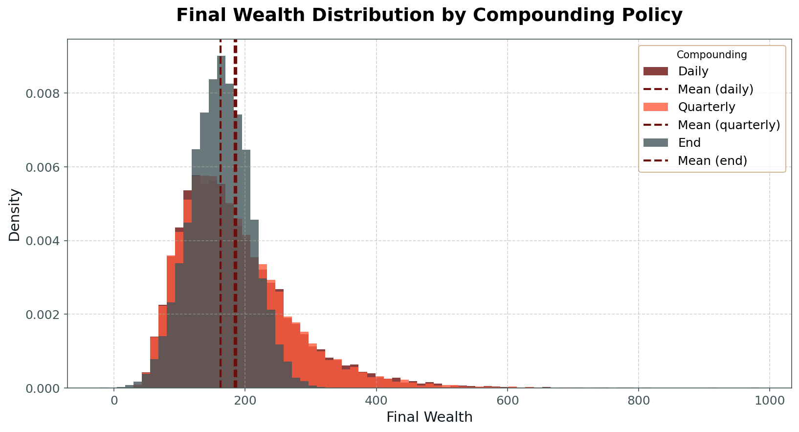
In practice, most real-world money machines fall somewhere between these extremes. Portfolios may maintain fixed position sizes on a daily basis, but adjust to new account values at monthly or quarterly intervals. This introduces intermediate degrees of compounding and path dependency, and alters both the distribution and predictability of long-run returns. Looking at an example wealth curve for the same underlying returns and different compounding policies in Fig 4, we can see how the compounded wealth curve has larger swings compared to the non-compounded curve, and that this amplification is larger on the upward side.

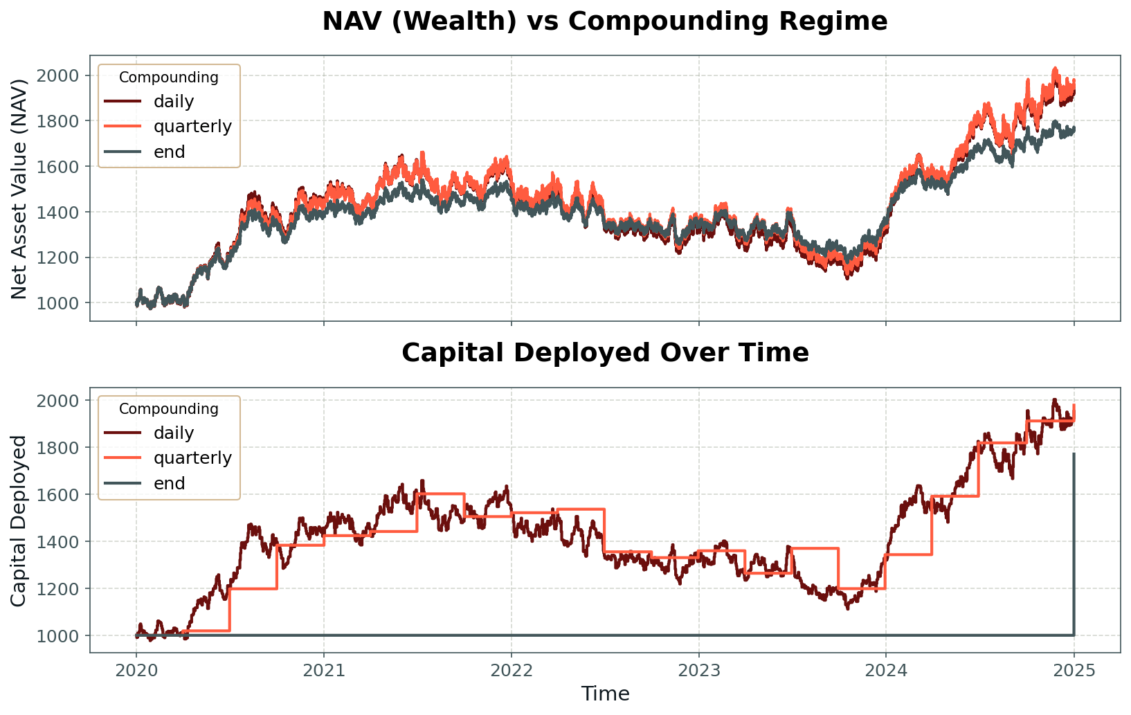
Empirically, compounding has a powerful effect on the distribution of outcomes. The positive skew of the compounded wealth distribution originates from the fundamental asymmetry of multiplicative returns: while losses are capped by the zero lower bound on wealth, gains remain unbounded. In addition, compounding introduces path dependency into the stream of returns measured in absolute terms, reducing the effective number of independent bets per unit of time and thereby diminishing the variance-reducing effect of diversification. This is visible when we simulate the money machine under varying compounding regimes and plot the resulting wealth distributions: full compounding produces fatter tails and more variability than arithmetic averaging, even with the same underlying daily return distribution (Fig 5).

It is also worth noting the conventions of professional portfolio management. Most asset managers and hedge funds do not compound their returns in the pure sense; instead, they operate within fixed risk budgets, typically defined by measures such as daily Value-at-Risk (VaR) or conditional VaR (cVaR). This approach seeks to avoid the path dependency of compounding, enabling a greater number of “independent bets” per unit of time, and bringing the real-world outcome closer to the ideal of the central limit theorem.

With these observations in hand, we can now examine trading frequency itself and assess under what conditions it becomes a genuine source of higher performance. The central limit theorem implies a natural reduction in the standard deviation of aggregate returns (without compounding) that scales with the square root of the number of independent bets. If we increase trading frequency—for example, moving from quarterly to weekly frequency, and if both the expected payout and volatility per bet scale in accordance with theory (mean return linearly with frequency, standard deviation with its square root), then the distribution of aggregate quarterly returns is unaffected by whether trades are executed weekly or quarterly. In such a scenario, we would be fundamentally indifferent to the choice of trading frequency. As previously discussed, more frequent compounding introduces greater path dependency and positive skew into the wealth distribution, but the diversification benefit from reduced volatility is exactly offset by our calibration. To create real value, higher frequency trading must deliver superior scaling of either expected return or risk (i.e., outperforming the central limit theorem), or exploit structural features of the market that are not captured by iid assumptions. This is both the challenge and the opportunity for professional traders who pursue higher frequency strategies.

We're all in this together

Thus far, we have, along with the classical conditions for the central limit theorem, assumed that returns are independent. In practice, however, returns often exhibit dependencies, whether across time, between strategies, or among assets and signals. Correlation, as the simplest form of linear statistical co-relationship, provides a direct lens through which to examine how such dependencies erode the effectiveness of diversification and weaken the conclusions of the central limit theorem.
In the cross-sectional case, considering multiple assets or strategies at the same point in time, positive correlations reduce the diversification benefit. Even if the marginal distributions of each strategy’s returns are identical, the portfolio’s aggregate volatility is higher when they tend to move together. This is the intuition behind correlation matrices in portfolio construction: the more independent the bets, the greater the risk reduction when combined.
In the time-series case, considering a single strategy or portfolio over time, autocorrelation plays a similar role. Here, the “bets” are sequential returns rather than concurrent ones. Positive autocorrelation means that a gain today is more likely to be followed by a gain tomorrow (and likewise for losses), while negative autocorrelation means reversals are more common. From the perspective of the CLT, positive autocorrelation has the same impact as positive cross-sectional correlation: it reduces the effective number of independent samples, slowing the rate at which the distribution of aggregated returns converges to normality.

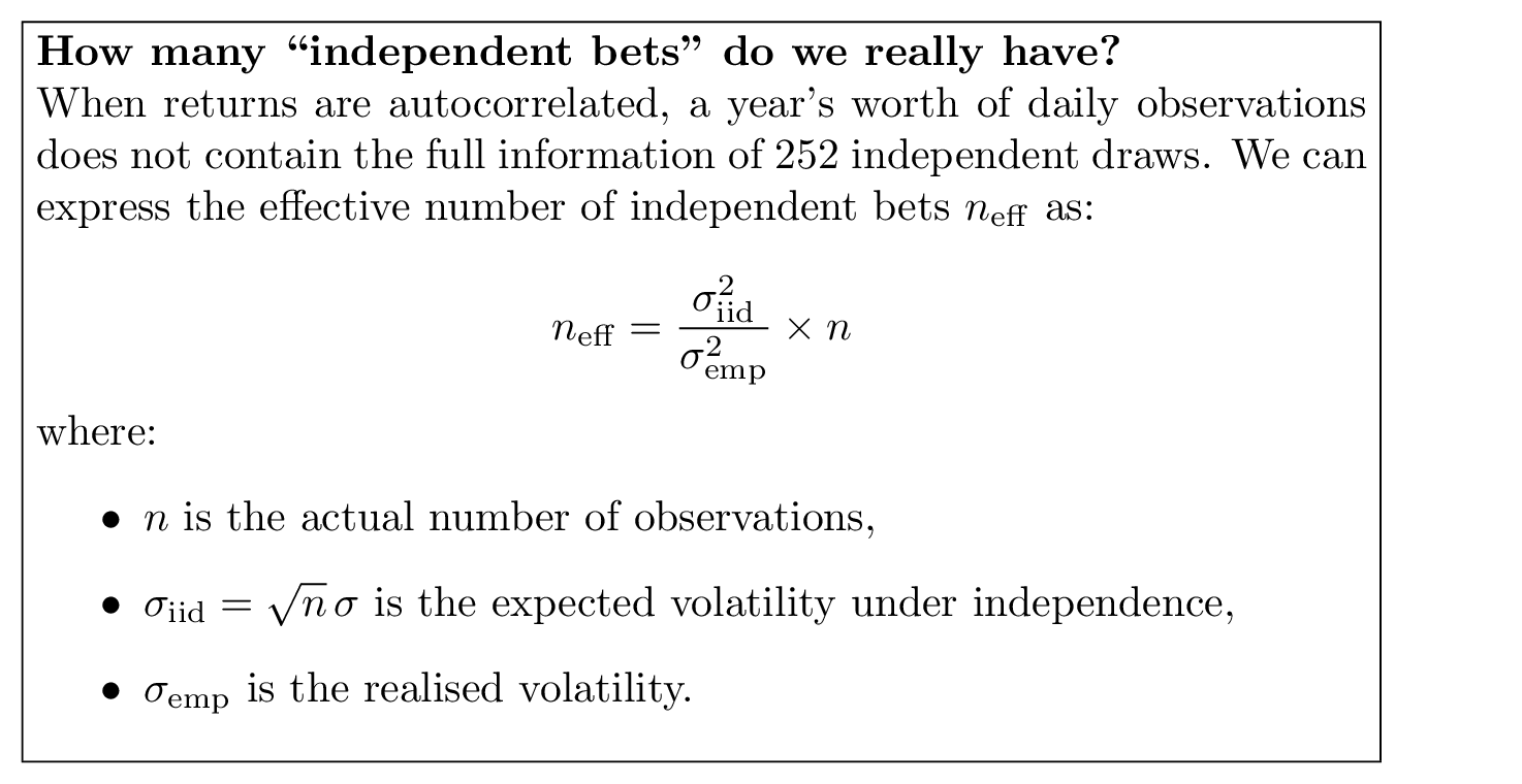
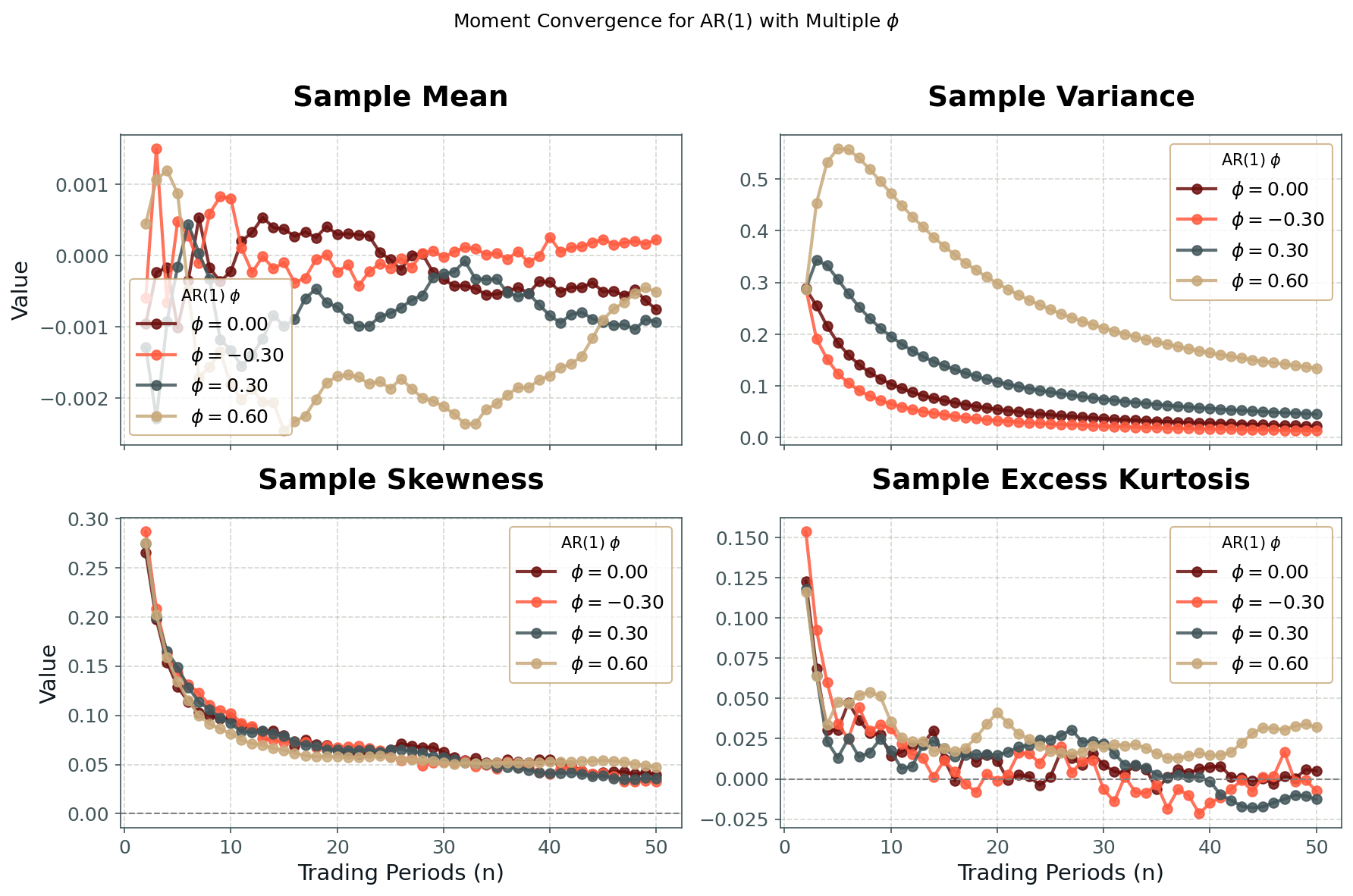
Figure 6 illustrates this effect for a simple AR(1) return process with varying degrees of autocorrelation. As autocorrelation increases, convergence of the first four moments (mean, variance, skewness, kurtosis) towards their CLT limits slows noticeably. The variance in particular declines more slowly than the 1/√n scaling of the independent case, reflecting the fact that successive returns are partially redundant observations.

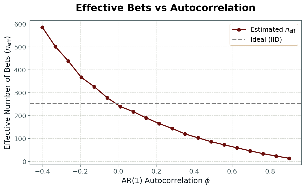
We can visualise this effect by plotting the effective number of independent bets against the degree of autocorrelation. As shown in Fig. 7, even modest positive autocorrelation sharply reduces the effective sample size. What looks like a year of 252 daily returns may, in practice, contain far fewer truly independent observations. This reduction directly weakens the diversification benefit and slows the convergence of return distributions toward normality.

A related, and very common, form of dependency in financial returns is volatility clustering. In clustered-volatility series, periods of high volatility tend to be followed by high volatility, and low volatility by low volatility, even if the direction of returns is unpredictable. This introduces another layer of dependency: not only are returns correlated through their signs or magnitudes, but the scale of returns changes over time in a persistent way. Volatility clustering reduces the effective number of independent observations in much the same way as autocorrelation, and it can distort inference if left unaccounted for.
In practice, most professional money machines manage volatility clustering through volatility targeting: adjusting position sizes dynamically to maintain a roughly constant expected volatility. This does not remove the clustering in the underlying process, but it normalises the scale of returns at the portfolio level, restoring comparability over time and mitigating some of the statistical consequences. Still, awareness of volatility clustering is important when interpreting back-tests or live performance—especially if the targeting process itself has lags or constraints that allow high-volatility episodes to bleed into realised returns.

Where this leaves us

In this first part we have seen how diversification, compounding, and dependencies shape the return streams of a money machine. Diversification narrows distributions and reduces risk, but its benefits are limited by compounding effects, correlation, and volatility clustering. These forces determine the broad statistical shape of a P&L stream, even before we introduce preferences or uncertainty.

So far, however, we have treated the underlying parameters—mean return, volatility, correlation—as if they were known and stable. In practice they are not. Estimates are noisy, regimes change, and learning about the process is itself part of the challenge.

In Part 2, we turn to this problem of uncertainty and learning. We will model parameters as random variables, show how beliefs update over time, and explore why the speed of learning can be just as valuable as the level of returns themselves.